Regression in Machine Learning

Regression is a supervised learning technique widely used in Machine Learning and Data Science. These kind of techniques aims to predict a continuous outcome variable (y) based on the values of one or more predictor variables and features (X), which can be continuous and/or discrete. Regression methods generally works by finding the mathematical relationship between the features and the outcome. When dealing with multiple predictors, the regression model is often represented as a multi-dimensional plane (also called hyperplane).

Unlike classification, which predicts a discrete category, regression quantifies the relationship between features, allowing us to predict a continuous outcome. Let's consider a practical example: If we want to predict the price of a house (a continuous variable), we might look at features such as size, location, number of rooms, construction materials, etc. A regression algorithm would find the best mathematical relationship between these features and the price of the house.

Uses of Regression

Regression models have incredibly versatile applications and find utility across a spectrum of fields. Let's delve into some areas where regression models are essentials:

• Finance: Regression models serve as powerful tools in the field of finance, particularly in risk assessment and financial forecasting. For example, with them analysts can predict a company's future earnings based on various financial indicators or forecast future stock prices based on historical data.

• Economics: Regression models are crucial in the field of economics. Economists employ them to forecast various economic indicators and measure the impact of changes in certain variables like employment rates or interest rates. For instance, economists could use regression to understand how a change in government policy might influence and affect the overall employment rate.

• Healthcare: This is one of the fields where regression models shine and have valuable applications. They can predict patient outcomes based on various factors such as age, weight, genetic predispositions, lifestyle, etc. They can also be used to understand the impact of different treatment approaches on patient recovery or even disease progression. For example, regression models could be used to predict the progression of a disease like diabetes based on various patient-specific factors.

• Marketing: In marketing, regression models are widely used for predictive tasks, such as predicting the success of marketing campaigns, forecasting sales, and understanding customers behavior. For instance, they can predict customer lifetime value based on purchase history, helping companies to optimize their customer retention strategies and approaches in future campaigns.

Regression Algorithms

There are various types of regression algorithms, each with its strengths, weaknesses, and suitability for different types of problems, some of them are:

• Linear Regression: One of the simplest forms of regression. It assumes a linear relationship between the predictors and the outcome variable.

• Polynomial Regression: This is an extension of linear regression, where the model is not restricted to a straight line and can fit polynomial curves to the data.

• Ridge and Lasso Regression: These are regularization techniques that help prevent overfitting in regression models. They do this by adding a penalty term to the cost function, which reduces the magnitude of the model coefficients.

• Decision Tree Regression: Decision trees can also be used for regression tasks, with the leaf nodes predicting continuous values.

• Support Vector Regression: This is the regression version of the Support Vector Machines (SVM), a robust and widely used algorithm in both classification and regression tasks.

• Random Forest and Gradient Boosting Regression: Ensemble techniques that combine predictions from multiple models to give a final prediction.

• Neural Network Regression: Neural networks can model complex non-linear relationships. They are especially useful for high-dimensional and complex data, where traditional regression techniques might struggle.

Regression models are a powerful tool in the hands of data scientists and analysts. They allow us to understand and quantify relationships between variables, make predictions about future data points, and even extrapolate trends outside the range of our current data. Being able to estimate the potential impact of different variables on an outcome can provide valuable insights for decision-making.

In future posts, I will dive deeper into these regression techniques, exploring how they work and implementing them using Python.

Read More

Data Encoding

In the field of data science, the quality and format of the data we work with are just as important as the algorithms and models we use. One of the crucial aspects of data preprocessing is Data Encoding, a process that transforms categorical data into a format that can be understood by machine learning algorithms.

Categorical data refers to variables that contain label values rather than numeric values. They are often divided into nominal (variables without order or priority) and ordinal (variables with some level of priority) categories. While this data can be insightful and necessary, many machine learning algorithms can only handle numerical inputs. This is where Data Encoding comes in. It converts these categorical variables into numerical values, allowing us to include this valuable information in the models we use.

Types of Data Encoding

There are several common types of Data Encoding, each with its own strengths and weaknesses. The choice of which to use often depends on the problem, the specific characteristics of the data and the requirements of the machine learning algorithm.

Nominal / One-Hot Encoding

The One-Hot Encoding, also called nominal encoding, is a widely used encoding technique for handling categorical variables. In this method, each category of is converted into a new binary column (values 0 or 1). This results in a sparse matrix where each row represents an observation and each column represents a unique category of the feature. The value is 1 if the category is present for that observation and 0 if not.

One-Hot Encoding is particularly useful for nominal data where no ordinal relationship exists. It allows the representation of categorical data in a way that can be understood by machine learning algorithms. However, it can lead to a high memory consumption and computational cost when the cardinality of the categorical variable is high, because it creates a new column for each unique category.

Now, let's see an example of how One-Hot Encoding can be implemented in Python.

First, we import the necessary libraries and create a pandas dataframe with two categorical features: Color and Shape. 

# Importing libraries
import pandas as pd
from sklearn.preprocessing import OneHotEncoder

# Creating a DataFrame with example data
data = {'Color': ['Red', 'Blue', 'Green', 'Yellow', 'Red', 'Green', 'Blue'],
        'Shape': ['Circular', 'Square', 'Square', 'Circular', 'Square', 'Circular', 'Square']}

df = pd.DataFrame(data)

# Displaying the DataFrame
print(df)

The created dataframe is:

Then, we define an instance of the OneHotEncoder class from the sklearn library. We apply this encoder to the dataframe using fit_transform, this method works by first learning the unique values of each feature (the fit part), and then transforming these values into a binary one-hot encoding (the transform part).

# Creating an instance of the OneHotEncoder
encoder = OneHotEncoder(sparse_output=False)
# Fitting and transforming the data
encoded_data = encoder.fit_transform(df)

Finally, we create and display a new dataframe with the encoded data.

# Creating a DataFrame with the encoded data
df_encoded = pd.DataFrame(encoded_data, columns=encoder.get_feature_names_out(df.columns))
# Displaying the encoded DataFrame
print(df_encoded)

The encoded dataframe resulted as:

Label Encoding

Label Encoding is another popular technique for encoding categorical variables. In this method, each unique category value is assigned an integer value. The assignment of integers is arbitrary and is usually based on the order of the categories in the feature.

Label Encoding is simple and efficient, making it a good choice for ordinal data and for nominal data with only two categories (binary data). However, it can introduce a potential issue for nominal data with more than two categories. The algorithm might misinterpret the numerical values as having an ordinal relationship, which can lead to poor performance or unexpected results.

Let's examine an example of Label Encoding implementation in Python.

We import the libraries and load the Iris dataset using the load_dataset function from the seaborn library. This is a classic dataset in machine learning and statistics. It includes measurements for 150 iris flowers from three different species (setosa, versicolor and virginica). 

# Importing libraries
import pandas as pd
import seaborn as sns
from sklearn.preprocessing import LabelEncoder

# Loading the iris dataset
iris = sns.load_dataset("iris")
# Displaying a sample of the dataset
iris.sample(5, random_state = 0)

A sample of the Iris dataset is shown below:

Then, we define an instance of the LabelEncoder class from the sklearn library. The fit_transform method is used to apply the encoder to the feature species.

# Creating an instance of the Label Encoder
label_encoder = LabelEncoder()
  
# Fitting and transforming the labels in column 'species'
iris_encoded = iris.copy()
iris_encoded['species']= label_encoder.fit_transform(iris_encoded['species'])

# Displaying a sample of the encoded dataset
iris_encoded.sample(5, random_state = 0)

The same sample of the Iris dataset, but with the feature species encoded, is:

Ordinal Encoding

Ordinal Encoding is a type of encoding that is similar to Label Encoding but with a key difference. In Ordinal Encoding, the assignment of integers to categories is not arbitrary. Instead, the integers are assigned in a way that respects the ordinal nature of the category.

For example, if a feature describes a rating as "low", "medium", or "high", ordinal encoding would assign the values 0, 1, and 2, respectively, preserving the order of the categories. This method is ideal for ordinal data, as it allows the model to understand the inherent order of the categories.

Let's explore an example of implementing Ordinal Encoding in Python.

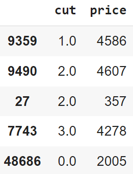
We import the libraries and load the cut and price attributes from the Diamonds dataset using the load_dataset function from the seaborn library.

# Importing libraries
import pandas as pd
import seaborn as sns
import numpy as np
from sklearn.preprocessing import OrdinalEncoder

# Loading the attributes "cut" and "price" from the diamonds dataset
diamonds = sns.load_dataset("diamonds")[["cut", "price"]]
# Displaying a sample of the dataset
diamonds.sample(5, random_state = 6)

Below is a sample of the dataset used:

Then, we create an instance of the OrdinalEncoder class from the sklearn library, by passing the categories of the cut feature as an argument. These categories were 'Fair', 'Good', 'Very Good', 'Premium' and 'Ideal', the ordinal encoder model assigned the numbers 0-4 to these categories in the order of their quality. The fit_transform method apply the encoder to the feature cut.

Below is the same sample of the dataset, but after applying the encoder:

Conclusion

In conclusion, data encoding is a crucial step in the data preprocessing pipeline, especially when dealing with categorical data. It allows us to transform non-numerical data into a format that can be understood and used by the machine learning algorithms.

In this post, we have explored several types of data encoding methods, including One-Hot Encoding, Label Encoding and Ordinal Encoding. Each of these methods has its own use cases and is appropriate in different circumstances. For example, One-Hot Encoding is useful when the categorical variables are nominal, while Label and Ordinal Encoding are beneficial when the categories have an inherent order.

Remember, the choice of encoding method can significantly impact the performance of the machine learning model. Therefore, it's essential to understand these methods and make an informed decision based on the nature of the data and the requirements of the model.

Read More

Drawing the Line: Understanding Decision Boundaries

In the domain of data science, classification problems are everywhere. From identifying spam emails to diagnosing diseases, Classification algorithms have transformed the way we make decisions. Understanding and visualizing decision boundaries offers significant insights into the behavior and performance of these algorithms.

A decision boundary is a significant concept, as it provides a visual interpretation of how different classification algorithms work. Selecting the right algorithm for a specific problem significantly impacts the classification performance, because no model is universally best for all problems. Therefore, it's imperative to compare different classification algorithms to understand which one has the best performance and generalization capacity.

In this blog post, I explore the concept of decision boundaries and compare the performance of three popular classification algorithms: K-Nearest Neighbors (KNN), Gaussian Naive Bayes, and Decision Tree. For more information about these models, refer to the respective posts here.

Understanding Decision Boundaries

A decision boundary, in the context of classification algorithms, is a hypersurface that effectively partitions the underlying feature space into two decision regions, each representing a different class. The geometry and complexity of these boundaries depend on the classification algorithm and can range from simple linear separators to convoluted hypersurfaces. 

By visualizing these decision boundaries, one can grasp how different algorithms partition the feature space and understand their classification logic. A straight boundary might suggest that an algorithm is making predictions based on a single feature, while a more complex boundary may indicate the use of multiple features. Understanding the nature of these boundaries also helps in comprehending the model's robustness, susceptibility to noise, and its potential for overfitting or underfitting.

Classification Algorithms to Compare

K-Nearest Neighbors: It's a simple and powerful classification method that works by comparing an unclassified sample with K similar samples in the training set. The unclassified sample is then assigned the most common class among its 'K' neighbors. KNN's decision boundaries can vary greatly with the choice of 'K' and distance metric, providing a flexible way to classify complex datasets. More information on this algorithm can be found here.

Gaussian Naive Bayes: These classifiers are based on applying Bayes' theorem, with strong independence assumptions between the features. It assumes that the data from each label is drawn from a simple Gaussian distribution. Despite its simplicity, Gaussian Naive Bayes can be surprisingly effective and is especially suitable for datasets with many features. It tends to produce decision boundaries that are quadratic. Refer to this link for more details.

Decision Tree: A decision tree is a flowchart-like structure where each internal node denotes a test on an attribute, each branch represents the outcome of a test, and each leaf node holds a class label. The decision boundaries are typically axis-aligned, partitioning the feature space into cuboids. Decision trees can handle both numerical and categorical data, making them a versatile choice for many classification problems. Learn more about decision trees here.

In the following section, I compare these three algorithms, examining their decision boundaries and computing their performance in terms of accuracy.

Visualizing Decision Boundaries

To visualize the decision boundary I implemented the machine learning models in Python using the scikit-learn library. I also developed functions to plot the decision boundaries and compute the accuracy scores of the models.

Importing Necessary Libraries

First, we need to import the essential Python libraries that were used throughout the project.

# Import necessary libraries
import pandas as pd
import numpy as np
import matplotlib.pyplot as plt
from matplotlib.colors import ListedColormap
import matplotlib.patches as mpatches
from sklearn.neighbors import KNeighborsClassifier
from sklearn.naive_bayes import GaussianNB
from sklearn.tree import DecisionTreeClassifier
from sklearn import datasets
from sklearn.model_selection import cross_val_score

Here we import the libraries pandas and numpy for handling and manipulating data, matplotlib for creating plots, sklearn for the machine learning algorithms, metrics and datasets.

Defining functions

We develop two functions: DecisionBoundaries and Cal_Acc.

The function DecisionBoundaries plots the decision boundaries for different classifiers on various datasets. It creates a grid of subplots where each row represents a specific dataset and each column represents a classifier. The first column in each row presents the datasets with their true labels.

# Function to Plot Decision Boundaries
def DecisionBoundaries(model_names, models, arr_datasets, arr_labels, size):

    h = 0.02  # step size in the mesh
    fig, axs = plt.subplots(len(arr_datasets), len(model_names) +1, figsize = size, facecolor='#F5F5F5')

    # Defining colormaps for visualizing the decision boundaries
    points_colormap = ListedColormap(['#FF0000', '#00FF00'])
    background_colormap = ListedColormap(['#FFAAAA', '#c2f0c2'])
    # Defining patches for the legend
    class0 = mpatches.Patch(color='#FF0000', label='0')
    class1 = mpatches.Patch(color='#00FF00', label='1')

    # Iterate through each dataset
    for i, (dataset, labels) in enumerate(zip(arr_datasets, arr_labels)):
        # Setting limits for the meshgrid
        x_min, x_max = dataset[:, 0].min() - 0.1*abs(dataset[:, 0].min()), dataset[:, 0].max() + 0.1*abs(dataset[:, 0].max())
        y_min, y_max = dataset[:, 1].min() - 0.1*abs(dataset[:, 1].min()), dataset[:, 1].max() + 0.1*abs(dataset[:, 1].max())
        xx, yy = np.meshgrid(np.arange(x_min, x_max, h), np.arange(y_min, y_max, h))
        # Displaying input data
        axs[i,0].set_facecolor('#F5F5F5')
        scatter = axs[i,0].scatter(dataset[:, 0], dataset[:, 1], c=labels, cmap=points_colormap, edgecolor='k')
        axs[i,0].legend(handles=scatter.legend_elements()[0], labels=['0', '1'], title = 'Classes')
        if i == 0:
          axs[i,0].set_title("Input Data")

        # Iterate through each model
        for j, (name, model) in enumerate(zip(model_names, models)):
            # Applying the model to generate decision regions
            model.fit(dataset, labels)
            decision_boundary = model.predict(np.c_[xx.ravel(), yy.ravel()])

            # Plotting the decision boundaries
            decision_boundary = decision_boundary.reshape(xx.shape)
            axs[i,j+1].set_facecolor('#F5F5F5')
            axs[i,j+1].pcolormesh(xx, yy, decision_boundary, cmap=background_colormap)
            # Plotting the data points
            scatter = axs[i,j+1].scatter(dataset[:, 0], dataset[:, 1], c=labels, cmap=points_colormap, edgecolor='k')
            axs[i,j+1].legend(handles=scatter.legend_elements()[0], labels=['0', '1'], title = 'Classes')

            # Adding title to each subplot
            if i == 0:
              axs[i,j+1].set_title(name)

The Cal_Acc function computes the average accuracy of each model on each dataset using 10-fold cross-validation. It stores the accuracy results in a pandas DataFrame for easier visualization and interpretation.

# Function to Calculate Average Accuracies using K-Fold Cross Validation
def Cal_Acc(model_names, models, dataset_names, arr_datasets, arr_labels):

    Accuracies = np.zeros((len(arr_datasets), len(model_names)))
    # Iterate through each dataset
    for i, (dataset, labels) in enumerate(zip(arr_datasets, arr_labels)):

        # Iterate through each model
        for j, model in enumerate(models):
            # Calculating cross-validation accuracy and storing in an array
            acc = cross_val_score(model, dataset, labels, cv=10, scoring='accuracy').mean()
            Accuracies[i, j] = round(acc, 5)

    # Generating a DataFrame from the accuracy array
    df_accuracies = pd.DataFrame(Accuracies, columns = model_names)
    df_accuracies.insert(0, "Datasets", dataset_names, True)

    return df_accuracies

Dataset Generation

We create three synthetic datasets, each presenting a different type of distribution and classification challenge: concentric circles (make_circles), half-moon shapes (make_moons), and two blobs (make_blobs). Each dataset have the corresponding set of labels.

# Generating Datasets
Dataset1, Labels1 = datasets.make_circles(n_samples=600, noise=0.13, factor = 0.5, random_state=0)
Dataset2, Labels2 = datasets.make_moons(n_samples=600, noise=0.22, random_state=0)
Dataset3, Labels3 = datasets.make_blobs(n_samples=600, centers = 2, cluster_std=1.3, random_state=0)

Then, we group them together in arrays.

# Grouping Datasets
arr_Datasets = [Dataset1, Dataset2, Dataset3]
arr_Labels = [Labels1, Labels2, Labels3]
dataset_names = ["Dataset 1", "Dataset 2", "Dataset 3"]

Defining Machine Learning Models

We define the classification models: K-Nearest Neighbors (KNN), Gaussian Naive Bayes, and Decision Tree. 

# Defining Models
KNN_model = KNeighborsClassifier(n_neighbors=5)
NaiveBayes_model = GaussianNB()
DecisionTree_model =  DecisionTreeClassifier(criterion = 'gini', splitter = 'best', random_state = 0)

We also group the models in an array.

# Grouping Models
models = [KNN_model, NaiveBayes_model, DecisionTree_model]
model_names = ["K-Nearest Neigbohrs", "Gaussian Naive-Bayes", "Decision Tree"]

Results

We use the functions to plot the decision boundaries and calculate the accuracies of the models, applying them to each dataset generated in previous sections.

# Plotting Decision Boundaries
DecisionBoundaries(model_names, models, arr_Datasets, arr_Labels, size = (18,10))

# Calculating Average Accuracies
accuracies = Cal_Acc(model_names, models, dataset_names, arr_Datasets, arr_Labels)

The graph containing the decision boundaries of each model and dataset is shown below:

The results for the accuracy scores of the models applied to each dataset were:

Conclusion

Understanding decision boundaries provides valuable insights into the behavior of classification models. It reveals how each model draws the 'line' between different classes, which can be a crucial factor in certain applications. In this blog post, we explored decision boundaries and implemented popular classification models, namely K-Nearest Neighbors (KNN), Gaussian Naive Bayes, and Decision Trees, to understand their decision-making process.

Through a comparative study, we demonstrated that each model has its strengths and weaknesses, and their performance can significantly vary depending on the complexity and distribution of the data. This underlines the importance of comprehending the underlying mechanisms of these models and applying this understanding in the model selection process.

Read More

Decision Trees for Classification

The Decision Tree algorithm is a powerful and versatile machine learning technique, it belongs to  supervised learning paradigm and is widely used for both Classification and Regression tasks, but is mainly used for classification problems. These algorithms work by creating a model that predicts the value of a target variable by learning simple decision rules based on the data features.

The importance of Decision Trees lies in their simplicity and interpretability. Unlike other machine learning algorithms, Decision Trees require little data preparation and can handle data which hasn't been normalized or encoded, as well as both categorical and numerical data. They also provide a clear indication of which fields are most important, making them a valuable tool for understanding complex datasets.

Decision Trees are fundamental components of Random Forests, which are among the most potent Machine Learning algorithms available today. In the real world, Decision Trees have a wide range of applications. They are used in the medical field for aiding in diagnosis, in finance to assess a potential investment risk, in retail to help predict a customer's likely purchases, and in many other fields.

Structure of Decision Trees

The structure of a Decision Tree is straightforward and intuitive. It consists of a root node, internal nodes, and leaf nodes. Each internal node represents a feature, each leaf node represents a class label, and each branch represents a rule. The topmost node in a Decision Tree is known as the root node. 

The tree starts at the root node and splits the data on the feature that results in the largest information gain (IG). In an iterative process, this splitting procedure is repeated at each child node until the leaves are pure. This means that all the samples at each node belong to the same class.

Metrics for Split Quality

There are many metrics used to evaluate the quality of a split in Decision Trees, some of which commonly used are Information Gain, Gini Impurity, and Entropy.

Entropy is a measure of the randomness or uncertainty, the goal of using entropy in a Decision Tree is to find and connect nodes with information that is most valuable for classification, which is done by minimizing the entropy, the formula of entropy is: which is the goal of the information gain criterion.

\begin{equation*} \mathbf{E} = \sum_{i=1}^{n}p_i \log_2 (p_i)  \end{equation*}

Information Gain is the reduction in entropy or impurity from a split. It measures how well a given attribute separates the training examples according to their target classification. It represents how much information a feature provides for the target variable, and this attribute with the highest information gain is chosen as the splitting feature at each node.

\begin{equation*} \mathbf{IG} = E_{parent} - E_{children}  \end{equation*}

Where $E_{parent}$ is the entropy of the parent node and $E_{children}$ represents the average entropy of the child nodes that follow this variable.

Gini Index is other alternative for splitting a decision tree. While the Entropy and Information Gain method focuses on purity and impurity in a node, the Gini Index measures the degree or probability for a particular variable being misclassified when it is randomly chosen. The formula for Gini Index is:

\begin{equation*} \mathbf{Gini} = 1 - \sum_{i=1}^{n}p_{i}{}^2  \end{equation*}

The lower the Gini Index, the lower the probability of misclassification, a Gini Impurity of 0 represents the best split.

Algorithms for Building Decision Trees

There are var popular algorithms used to build Decision Trees, including CART (Classification and Regression Trees), ID3 (Iterative Dichotomiser 3), and C4.5.

• CART: The CART algorithm is a binary tree algorithm, meaning that each parent node splits into exactly two child nodes. It can handle both numerical and categorical variables and also can be used for both classification and regression tasks. CART uses the Gini Index as a metric to create decision points for classification tasks, and mean squared error for regression tasks.

• ID3: It uses a top-down, greedy approach to construct a decision tree. It selects the best attribute to place at the root node based on the Information Gain metric. The ID3 algorithm can handle categorical input attributes well, but struggles with continuous attributes. It also doesn't handle missing values, so any missing data needs to be preprocessed before to be used in an ID3 algorithm.

• C4.5: This algorithm is an extension of ID3 that adjusts the Information Gain using a "Gain Ratio" to handle the bias towards attributes with many outcomes. It can handle both continuous and categorical attributes, and also allows for missing feature values. The C4.5 model includes a pruning step, where it uses a statistical test to estimate whether expanding or collapsing some branches can improve its predictions, which helps to avoid overfitting.

Implementing algorithm in Python

In this section, I explain an implementation of the Decision Tree algorithm in Python using the scikit-learn library. Here I use the Iris dataset, which is a multivariate dataset introduced by the British statistician and biologist Ronald Fisher in his 1936 paper. The task is building a Decision Tree model to classify the iris species based on their properties.

Importing Libraries

First, we import the libraries for this script, which includes:

# Importing libraries
import numpy as np
import pandas as pd
from sklearn.datasets import load_iris
from sklearn.model_selection import train_test_split
from sklearn.tree import DecisionTreeClassifier, export_graphviz
from sklearn.metrics import accuracy_score
import matplotlib.pyplot as plt
from graphviz import Source

• numpy: It adds support for multi-dimensional arrays and matrices, along with a large collection of high-level mathematical functions to operate on these arrays.

• pandas: Library for data manipulation and analysis. It offers data structures and operations for manipulating numerical tables and time series.

• sklearn: It is a machine learning library for Python. It features various machine learning algorithms and also supports Python's numerical and scientific libraries. We specifically imported the load_iris function for loading the Iris dataset, train_test_split for splitting our data into train and test sets, DecisionTreeClassifier for building the Decision Tree model, export_graphviz for exporting the tree in a Graphviz format, and accuracy_score for calculating the accuracy of the model.

• matplotlib: It is a visualization library in Python for creating static, animated, and interactive visualizations, as well as drawing attractive and informative statistical graphs.

• Graphviz: This is an open-source graph visualization software. It is used to represent structural information as diagrams of abstract graphs and networks. In this case, it is used to plot the tree diagram of the trained model.

Loading the Iris Dataset

This dataset is freely available and built into the scikit-learn library. It includes three iris species (setosa, versicolor and virginica) with 50 samples each, as well as some properties about each flower (sepal length, sepal width, petal length and petal width). We first load this dataset and split it into input features X and the target variable y. The input features are the measurements of each flower and the target variable is the species of the flower.

# Loading the Iris dataset
iris = load_iris()
# Splitting the data into input features (X) and target variable (y)
X = iris.data
y = iris.target

Next, we create a Pandas dataframe with the data and the column names. This allows us to easily manipulate and explore the data. 

# Creating a Pandas DataFrame with the data and the column names
df = pd.DataFrame(data=X, columns=iris.feature_names)
# Adding the target variable column to the DataFrame
df['target'] = y

To make the data more understandable, we map the integer values of the target variable to the names of the Iris species.

# Creating a dictionary to map the integer label values to the class names
class_mapping = {0: 'setosa', 1: 'versicolor', 2: 'virginica'}
# Map the integer label values to the class names
df['target'] = df['target'].map(class_mapping)

Finally, we print out a random sample of 5 rows from our dataset. This is useful to get a quick overview of the data we are working with.

df.sample(n = 5, random_state = 0)

The random sample is shown below:

Applying the Decision Tree Model

Now that we have loaded the dataset, we can move on to applying the Decision Tree model. First, we split the data into train and test sets. This allows us to evaluate the performance of our model on unseen data. We use the train_test_split function from scikit-learn library, resulting that 25% of the samples belong to test set and 75% to train set.

# Split the data into training and testing sets
X_train, X_test, y_train, y_test = train_test_split(X, y, test_size=0.25, random_state=0)

Next, we create an instance of the DecisionTreeClassifier and train it using the training dataset.

# Creating an instance of DecisionTreeClassifier
decision_tree = DecisionTreeClassifier(criterion = 'gini', splitter = 'best', random_state = 0)
# Training the model using the train set
decision_tree.fit(X_train, y_train)

Once the model is trained, we apply it to make predictions on the test data. We also calculate the accuracy score to evaluate the performance of the model.

# Make predictions on the test set
y_pred = decision_tree.predict(X_test)
# Computing the accuracy of the model
accuracy = accuracy_score(y_test, y_pred)
print("The accuracy is:", accuracy)

The resulting accuracy of the models is 0.974, which indicates a good performance of the model.

Understanding the Structure of the Tree

One of the advantages of Decision Trees is that they are relatively easy to interpret. We can visualize the trained Decision Tree model using sklearn and the graphviz libraries.

# Generating a Graphviz representation of the Decision Tree
dot_data = export_graphviz(decision_tree, out_file=None, feature_names=iris.feature_names, class_names=iris.target_names, rounded=True)
# Creating a graph from the Graphviz representation
graph = Source(dot_data)
# Displaying the graph
graph

The export_graphviz function generates a Graphviz representation of the Decision Tree, which is a text language for describing graphs. Then, we use the Source function from the graphviz library to create a graph from the Graphviz representation of the Decision Tree. Finally, we display the graph, which is below:

Visualizing Feature Importance

Another advantage of Decision Trees is that they can compute the relative importance of features. This can be very useful in understanding which features are the most influential in making the predictions.

# Get the feature importances
importances = decision_tree.feature_importances_

# Creating a bar plot to visualize the feature importances
plt.rcParams['font.size'] = '12'
fig, ax = plt.subplots(figsize=(8,6), facecolor='#F5F5F5')
ax.set_facecolor('#F5F5F5')
bars = ax.bar(range(len(importances)), importances, tick_label=iris.feature_names)
ax.set_ylabel('Importance')
ax.set_title('Importance of features in decision tree model')
ax.set_xticklabels(iris.feature_names, rotation=45)

# Adding the value above each bar
for bar in bars:
    yval = bar.get_height()
    ax.text(bar.get_x() + bar.get_width()/2, yval, round(yval, 4), ha='center', va='bottom')

plt.show()

The feature_importances_ attribute of the model gives us the importance of each feature. These importances were computed as the total reduction of the criterion (Gini) brought by that feature. Then, we plot these feature importances on a bar plot for easy visualization.

This graph indicates that sepal length was not used in the decision-making process of the model, as it have an importance of 0.0. Sepal width, with an importance of 0.0201, played a minor role. But, the petal length and petal width features were the most influential in the decision-making process, with importances of 0.3993 and 0.5806, respectively. This suggests that these two features contributed the most to the reduction of impurity in the nodes, in other words, they are the most important features for the Decision Tree model.

Training a New Decision Tree Model with less Features

Given the importance scores that we obtained from the initial Decision Tree model, we showed that petal length and petal width are the most influential features in classifying the Iris species. To illustrate the impact of these features, we train a new Decision Tree model using only these two features.

We create new training and testing sets that only include the petal length and petal width features.

# Selecting only the 'petal length' and 'petal width' features for training and testing
X_train_reduced = X_train[:, 2:4]
X_test_reduced = X_test[:, 2:4]

Then, we define a new instance of the DecisionTreeClassifier and train it using the reduced-features training data.

# Creating a new DecisionTreeClassifier model
decision_tree_2 = DecisionTreeClassifier(criterion = 'gini', splitter = 'best', random_state = 0)
# Train the new model using the reduced training set
decision_tree_2.fit(X_train_reduced, y_train)

Finally, we compute the accuracy of the new model.

# Make predictions on the reduced testing set
y_pred_2 = decision_tree_2.predict(X_test_reduced)
# Computing the accuracy of the new model
accuracy_2 = accuracy_score(y_test, y_pred_2)
print("The accuracy of the new model is:", accuracy_2)

The accuracy of this new model, which only uses the petal length and petal width features, is 0.947. This is slightly lower than the accuracy of the initial model, which was 0.973. But, it's important to notice that this reduction is minimal.

Moreover, the fact that we are able to achieve nearly the same level of accuracy while reducing the number of features by half is quite significant. In larger, more complex datasets, reducing the dimensionality of the data can lead to substantial computational savings and can also help to mitigate the risk of overfitting.

Conclusion

In this post, we have explored the Decision Tree algorithm and its application in classification tasks. Through our hands-on implementation with the Iris dataset, we have seen how the model can be trained, how predictions can be made, and how the model's performance can be evaluated. We have also discovered the power of feature selection, by focusing on the most influential features, we were able to create a more efficient model that maintained nearly the same level of accuracy. This highlights the balance between model complexity and performance, a key consideration in machine learning.

In conclusion, we have learned about the power and importance of Decision Tree models, their simplicity, interpretability, and versatility make them a valuable tool in any data scientist's toolkit.

Read More

Gaussian Naive Bayes

Naive Bayes is a fundamental Classification algorithm in the field of machine learning and data science. This probabilistic model, rooted in the principles of Bayesian statistics, is famous and useful for its efficiency, simplicity, and surprisingly robust performance across a wide array of applications. Naive Bayes classifier is based on the Bayes' theorem, which is a principle in probability theory and statistics that describes the relationship of conditional probabilities of statistical quantities, in other words, it provides a way to calculate the probability of an event (variable) based on prior knowledge of another variable. 

The naive term in Naive Bayes refers to the assumption that all features in the dataset used for classification are mutually independent, this assumption simplifies the calculations for the posterior probabilities and makes the algorithm computationally efficient. Although this assumption is not common in real-world data, the Naive Bayes classifier often delivers robust performance, even when there is no independence among features.

There are several types of Naive Bayes models, including Gaussian Naive Bayes, Multinomial Naive Bayes, and Bernoulli Naive Bayes. Each type is suited to different kinds of data, In this post, I focus on the Gaussian Naive Bayes classifier, which assumes that the features follow a normal distribution. This variant is particularly useful when dealing with continuous data. 

How does the Gaussian Naive Bayes classifier work?

The Gaussian Naive Bayes classifier operates under the framework of Bayes' theorem, which in its simplest form can be expressed as:

\begin{equation*} \mathbf{P} \left(Y | X \right)= \frac {\mathbf{P} \left(X | Y \right) \mathbf{P} \left( Y \right)} {\mathbf{P} \left( X \right)} \end{equation*}

In the context of the Gaussian Naive Bayes classifier, Y and X are events where Y is the hypothesis (class label) and X is the evidence (features). $\mathbf{P} \left(Y | X \right)$ is the posterior probability, $\mathbf{P} \left(X | Y \right)$ is the likelihood, $\mathbf{P} \left(Y \right)$ is the prior probability, and $\mathbf{P} \left(X \right)$ is the evidence.

• Posterior probability $P \left(Y | X \right)$: It can be understood as the probability that an instance X (data point with specific features values) belongs to class Y.

• Likelihood $P \left(X | Y \right)$: It can be understood as the probability that, given a certain class label Y, the observed features have been X. In the Gaussian Naive Bayes classifier, this is calculated using the Gaussian (normal) distribution, hence the name.

• Prior probability $P \left(Y \right)$: It is the initial probability of an specific class Y, calculated as the proportion of samples of that class in the training set.

• Evidence $P \left(X \right)$: It is the total probability of the features X. In practice, this term is often ignored during the calculation, because it doesn't affect which class has the highest probability.

The pseudocode is described in the next image, which provides an outline of the basic Naive Bayes algorithm for classification.

Python Implementation

According to each dataset, the selection process for the number of neighbors K may be different. In this post the number K will be taken as arbitrary, but in a future post I'll talk about how to correctly select the number K.

Importing Libraries

First, we import the necessary libraries for the code, which includes:

import numpy as np
import seaborn as sns
import matplotlib.pyplot as plt
from matplotlib.colors import ListedColormap
from sklearn.naive_bayes import GaussianNB
from sklearn.metrics import confusion_matrix
from sklearn import datasets
from sklearn.model_selection import train_test_split
from sklearn.metrics import accuracy_score

• numpy: Provides mathematical functions to operate on arrays.

• sklearn: One of the most popular libraries for machine learning in Python. It features many machine learning algorithms, including the Naive Bayes algorithm (imported as GaussianNB). It also provides tools for model fitting, data preprocessing, model selection, model evaluation and other utilities.

• seaborn and matplotlib: These are visualization libraries in Python for creating static, animated, and interactive visualizations, as well as drawing attractive and informative statistical graphs.

Defining Functions

Now that we have imported the libraries, we can proceed to implement the Naive Bayes algorithm. We define two functions: calculate_parameters and naive_bayes.

# This function calculates the means, variances and prior probabilities
def calculate_parameters(X, y):
    unique_labels = np.unique(y)
    prior_probs = []
    means = []
    variances = []
    for label in unique_labels:
        # Calculating the prior probability of the label
        prob = np.count_nonzero(y == label)/len(y)
        prior_probs.append(prob)
        # Calculating the mean of the features
        mean = X[y==label].mean(axis = 0)
        means.append(mean)
        # Calculating the variance of the features
        variance = X[y==label].var(axis = 0)
        variances.append(variance)
    return np.array(means), np.array(variances), np.array(prior_probs)


# This function apply the Gaussian Naive Bayes algorithm to a test dataset
def naive_bayes(Test_Dataset, Train_Dataset, Train_Labels):
    means, variances, prior_probs = calculate_parameters(Train_Dataset, Train_Labels)
    Predicted_Labels = []

    # Classifying the test dataset
    for x in Test_Dataset:
        post_probs = []
        for i in range(len(prior_probs)):
            # Calculating P(xi | y) for each feature xi
            numerator = np.exp( -(x-means[i])**2 / (2 * variances[i]) )
            denominator = np.sqrt(2 * np.pi * variances[i])
            # Calculating P(x | y)
            p_x_given_y = np.prod(numerator/denominator)
            # Calculating P(y | X) for the class y
            prob_class_i = p_x_given_y*prior_probs[i]
            post_probs.append(prob_class_i)

        # Assigning the class with the highest posterior probability
        probable_class = np.argmax(post_probs)
        Predicted_Labels.append(probable_class)

    return np.array(Predicted_Labels)

The calculate_parameters function takes the training dataset and the corresponding labels as inputs. It calculates the mean and variance for each feature for each class, as well as the prior probability of each class. These parameters are used later when applying the Naive Bayes algorithm.

Next, we define the naive_bayes function, which applies the Naive Bayes algorithm to a test dataset. It takes the test dataset, the training dataset, and the training labels as inputs, and returns the predicted labels for the test dataset. This function calculates the posterior probability for each class for each data point in the test set, based on the parameters calculated by the calculate_parameters function. It then assigns the class with the highest posterior probability to each data point.

Generating and Visualizing Dataset

Now that we have the Naive Bayes classifier ready, we need a dataset to apply it. For this post, we generate a synthetic dataset using the make_circles function from the sklearn library. This function generates a large circle containing a smaller circle in two dimensions. We can control the number of data points and the amount of noise in the data.

# Setting parameters for the dataset
n_points = 3500 # Number of data points
noise = 0.12 # Standard deviation of Gaussian noise added to the data
color_map = ListedColormap(['mediumseagreen','mediumblue']) # Color map for the two classes

# Creating dataset
X,y = datasets.make_circles(n_samples=n_points, noise=noise, factor = 0.6, random_state=0)

After generating the dataset, we use matplotlib to create a scatter plot of the data points. The two classes are represented by different colors.

# Plotting generated dataset
plt.rcParams['font.size'] = '12'
fig, ax = plt.subplots(figsize=(8,6), facecolor='#F5F5F5')
ax.set_facecolor('#F5F5F5')
# Creating a scatter plot
scatter = ax.scatter(X[:, 0], X[:, 1], c=y, s=50, cmap=color_map, alpha = 0.4)
# Adding a legend to the plot
ax.legend(handles=scatter.legend_elements()[0], labels=['0', '1'], title = 'Classes')
ax.set_title("Generated Dataset", fontsize=15)

Splitting the Dataset for Train and Test

After generating the dataset, the next step is to split it into a train set and a test set, the first is used to train the Naive Bayes classifier (dataset used for calculate the means, variances and prior probabilities), while the second is used to evaluate the classifier's performance on new data. A common practice is to allocate 75% of the dataset to the train set and 25% to the test set.

# Splitting the dataset into a train set and a test set
X_train, X_test, y_train, y_test = train_test_split(X, y, test_size=0.25, random_state=0)

# Creating a figure with two subplots
fig, ax = plt.subplots(1,2, figsize=(14,5), facecolor='#F5F5F5')
# Plotting the train set
ax[0].set_facecolor('#F5F5F5')
scatter = ax[0].scatter(X_train[:, 0], X_train[:, 1], c=y_train, s=50, cmap=color_map, alpha = 0.4)
ax[0].legend(handles=scatter.legend_elements()[0], labels=['0', '1'], title = 'Classes')
ax[0].set_title("Train Dataset", fontsize=14)
# Plotting the test set
ax[1].set_facecolor('#F5F5F5')
scatter = ax[1].scatter(X_test[:, 0], X_test[:, 1], c=y_test, s=50, cmap=color_map, alpha = 0.4)
ax[1].legend(handles=scatter.legend_elements()[0], labels=['0', '1'], title = 'Classes')
ax[1].set_title("Test Dataset", fontsize=14)

We use the train_test_split function from the sklearn library to perform this split. This function shuffles the dataset and then splits it into train and test sets. Then, we create scatter plots to visualize both sets using the matplotlib library. These plots are shown below:

Applying Naive Bayes Algorithm

We already have the dataset and the Naive Bayes classifier, so we can apply this classifier to the dataset and evaluate its performance.

The naive_bayes function takes the test set, the train set and the train labels as inputs, and returns the predicted labels for the test set as output. We then calculate the accuracy of the predictions using the accuracy_score function from sklearn.

# Applying Naive Bayes algorithm
y_pred = naive_bayes(X_test, X_train, y_train)
print("The accuracy is:", accuracy_score(y_test, y_pred))

We can also use the GaussianNB model from the library sklearn. For this, we create a classifier object, then we fit it to the train set and finally predict the labels for the test set. The accuracy of these predictions is also calculated using the accuracy_score function.

# Applying Naive Bayes algorithm using model from Sklearn
bayes_sklearn = GaussianNB()
bayes_sklearn.fit(X_train, y_train)
y_pred = bayes_sklearn.predict(X_test)
print("The accuracy is:", accuracy_score(y_test, y_pred))

For both alternatives, the accuracy of the models is 0.95. 

After making the predictions, we create a confusion matrix using the confusion_matrix function from sklearn. The confusion matrix is a table that is often used to describe the performance of a classification model on a test set for which the true values are known. Then, we visualize the confusion matrix using a heatmap from the seaborn library.

# Creating a confusion matrix
cm = confusion_matrix(y_test, y_pred)
# Visualizing the confusion matrix using a heatmap
fig, ax = plt.subplots(figsize=(7,5), facecolor='#F5F5F5')
ax = sns.heatmap(cm, annot=True, fmt="d", cmap="YlOrBr", annot_kws={"size": 16})
ax.set_xlabel('Predicted labels', fontsize=14)
ax.set_ylabel('True labels', fontsize=14)
ax.set_xticklabels(['Class 0', 'Class 1'], fontsize=13)
ax.set_yticklabels(['Class 0', 'Class 1'], fontsize=13)
plt.show()

The confusion matrix shows that for the class 0, 423 points are classified correctly and 10 points are classified incorrectly. For the class 1, 410 points are classified correctly and 32 points are classified incorrectly. This indicates that the Naive Bayes classifier have a high accuracy. The confusion matrix is shown below:

Bonus: Visualizing the Predicted Labels

After applying the Naive Bayes classifier and evaluating its performance, we plot the test set with the correct labels and the predicted labels. It helps for a visual understanding of how well the classifier works.

We create two scatter plots: one for the test set with the correct labels, and another one for the test set with the predicted labels.

# Creating a figure and a set of subplots
fig, ax = plt.subplots(1,2, figsize=(14,5), facecolor='#F5F5F5')

# Plotting the test set with the correct labels
ax[0].set_facecolor('#F5F5F5')
scatter = ax[0].scatter(X_test[:, 0], X_test[:, 1], c=y_test, s=50, cmap=color_map, alpha = 0.4)
ax[0].legend(handles=scatter.legend_elements()[0], labels=['0', '1'], title = 'Classes')
ax[0].set_title("Correct Classes", fontsize=14)

# Creating a new color map for the predicted labels
color_map2 = ListedColormap(['mediumseagreen','mediumblue', 'firebrick'])
# Finding the indices of the points that were classified incorrectly
incorrect_indices = np.where(y_pred != y_test)[0]
# The labels of the points that were classified incorrectly are set to 2
y_plot = y_pred.copy()
y_plot[incorrect_indices] = 2

# Plotting the test set with the predicted labels
ax[1].set_facecolor('#F5F5F5')
scatter = ax[1].scatter(X_test[:, 0], X_test[:, 1], c=y_plot, s=50, cmap=color_map2, alpha = 0.4)
ax[1].legend(handles=scatter.legend_elements()[0], labels=['0', '1', 'Incorrect'], title = 'Classes')
ax[1].set_title("Predicted Classes", fontsize=14)

These plots are as follows:

In the second plot, the red points are those that were incorrectly classified by the model.

As we have shown, the Naive Bayes algorithm is a powerful and efficient tool for classification tasks. Despite its simplicity and the "naive" assumption of feature independence, it often performs surprisingly well in practice, even when the independence assumption is violated. Its efficiency and scalability make it particularly suitable for large datasets and applications where speed is crucial.

Through this post, we have seen how the Naive Bayes model can be implemented from scratch and applied to a synthetic dataset. We have also compared its performance with the implementation provided by the sklearn library. This exploration has demonstrated the practicality and effectiveness of the Naive Bayes algorithm. As with any machine learning model, it's important to understand its strengths and limitations, in order to consider them when we select an algorithm for a specific task.

Read More